
Trace 790,000 Building Outlines in Under an Hour: Preparing Satellite Imagery for AI Training on a 100-Node HPC Auto Scale Cluster
Use a Slurm job array on 100 small RONIN nodes to trace 790,221 building outlines in 14,896 satellite tiles. Detection takes 49 minutes, and a run costs about $8 USD.



Everyone wants to talk about training the model. Nobody wants to talk about the weeks before that, when you are checking, labelling and cleaning a mountain of images so the model has something good to learn from.
So let's make that part fast. In this tutorial, we will take 14,896 open satellite tiles of Atlanta, find and outline every building in every tile, check the results against hand-drawn labels, and save clean, ready-to-use labels to a RONIN bucket. We will do it with 100 small, cheap compute nodes that switch themselves on when the work arrives and off again when it is done.
In our test run, the detection work took 49 minutes and traced 790,221 building outlines. That is detections across 14 views of the same 1,064 locations, which hold about 65,600 unique labelled buildings. A run like this costs only $8 USD.
This guide is for researchers who are comfortable in a Linux terminal and want to see what a job array on an HPC Auto Scale Cluster can do. If you are new to the clusters, start with Meet the New HPC Auto Scale Clusters.
What you will build
Here is the whole pipeline at a glance. One head node does the downloading and the uploading. 100 compute nodes do the heavy lifting in between.
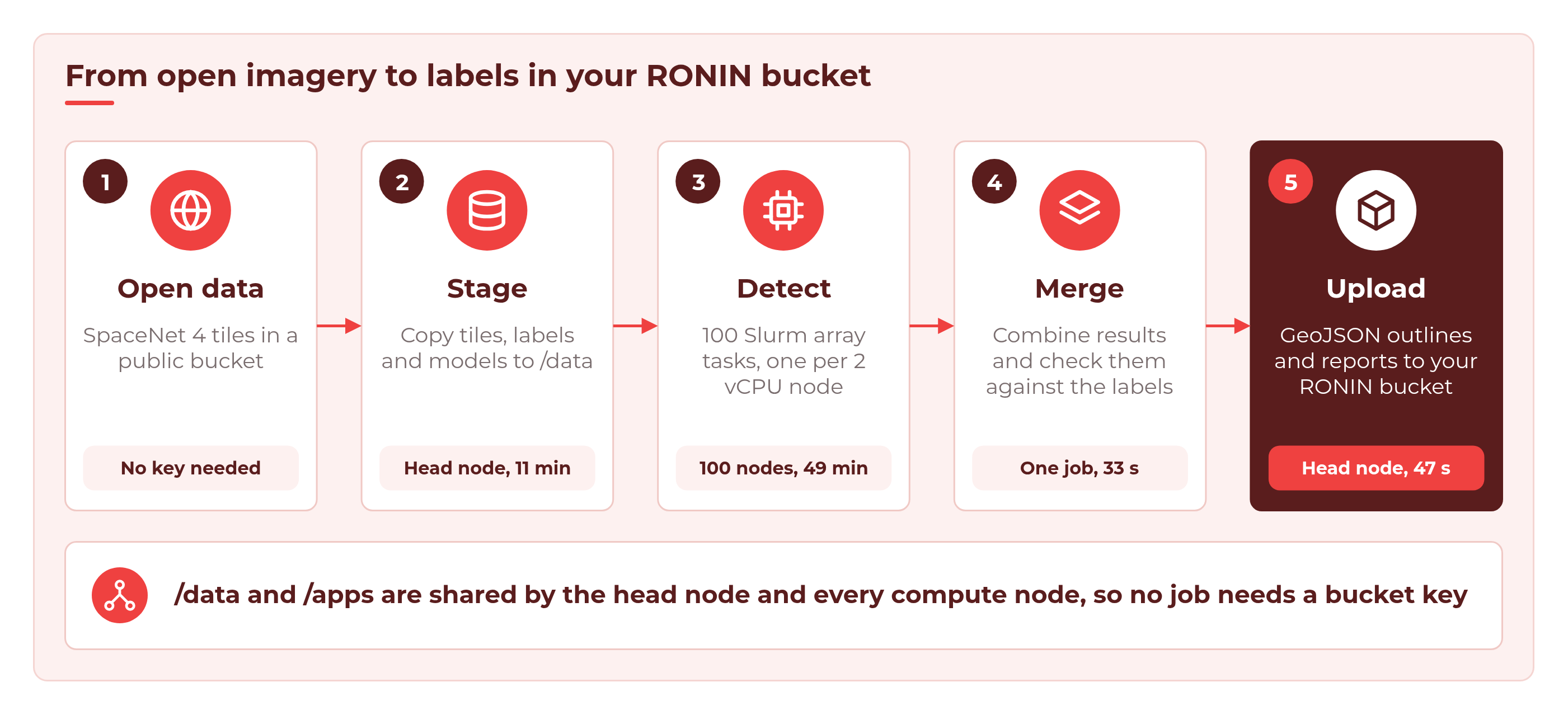
By the end you will have:
- a GeoJSON file of building outlines for every tile, which you can open in QGIS or geojson.io
- a building count and area for every tile, in one CSV
- a quality report that compares what the models found with what SpaceNet's annotators drew by hand
- a few overlay images so you can check the results with your own eyes
- all of it in a RONIN bucket, ready for your training pipeline
Why buildings, and why so many angles?
We are using SpaceNet 4: Off-Nadir Buildings. SpaceNet photographed the same 1,064 places in Atlanta 27 times, from almost straight down (7 degrees off nadir) to very oblique (54 degrees). We process 14 of those viewing angles, so 14 x 1,064 = 14,896 tiles of 900 x 900 pixels, resampled to 0.5 m per pixel. That is about 90 GB of imagery.
For every tile, three pretrained SpaceNet 4 building models score each pixel. They are U-Net neural networks, and their weights are published in the same public bucket. We average their scores, and every separate blob of building pixels becomes one building outline. It is a simple, CPU-only detector, and each tile keeps a 2 vCPU node busy for about 15 seconds. 15,000 of those in a row would take 2.6 days on one node. Spread over 100 nodes, it takes under an hour.
Before you begin
You will need:
- A RONIN project. Anyone in the project can create, edit, package and open clusters, just like machines.
- Enough EC2 vCPU quota for about 208 vCPUs (100 nodes x 2 vCPUs, plus an 8 vCPU head node). If you are not sure, ask your RONIN admin to check the Service Quota screen.
- The latest RONIN LINK on your computer, to connect to the cluster and open Grafana.
- The scripts in this tutorial. RONIN does not host or provide scripts, so every script you need is printed in full in the Full scripts section at the end of this post. You create each file by copying and pasting it.
No AWS account or keys are needed to download the data from the SpaceNet dataset on the Registry of Open Data on AWS. You only need a key at the very end, to upload to your own bucket.
Everything else is linked rather than provided. The imagery, labels and model weights come from the SpaceNet dataset above. You install the AWS CLI in Step 3. The Python packages (PyTorch, torchvision, NumPy, SciPy, rasterio, Shapely and Pillow) are downloaded and installed for you by the setup script.
Step 1: Launch the cluster
In your project, open Auto Scale Clusters from the left menu and click + NEW AUTO SCALE CLUSTER. Give your cluster a name, choose or create an SSH key, then set up the nodes.
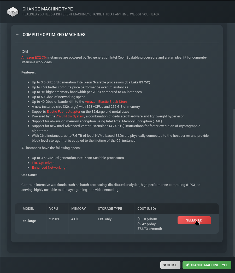
Compute nodes. Click CHANGE under compute nodes, find the C6i family in the compute machines section and select c6i.large (2 vCPUs, 4 GiB, $0.10 an hour). Then click CHANGE MACHINE TYPE. Leave hyperthreading enabled (the default). Our job script asks for 2 CPUs per task, and with hyperthreading off a c6i.large offers only 1 CPU, so Slurm would reject every task.
Head node. We used an m6i.2xlarge (8 vCPUs, 32 GiB). The head node does more than usual in this tutorial: it downloads 90 GB of tiles and shares /data with all 100 compute nodes at once, so it pays to give it some network and CPU headroom.
Storage. Set the DATA drive to at least 120 GB (we used 250 GB). The tiles take about 90 GB, plus models, labels and results. The APPS drive can stay at 20 GB.
Capacity. Set Min nodes to 0 and Max nodes to 100. Watch the forecast tiles update as you go.
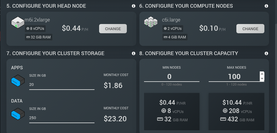
The wizard rounds its prices. At list price, 100 nodes plus the head node come to about $10.54 an hour, and the Cost tab showed about $10.59 an hour once the drives were included.
The forecast tells the story of this whole tutorial. With Min nodes at 0, an idle cluster costs about the same as the head node alone. You only pay the $10.44 an hour rate while all 100 nodes are actually working.
Then launch your cluster.

Step 2: Create a bucket for the results
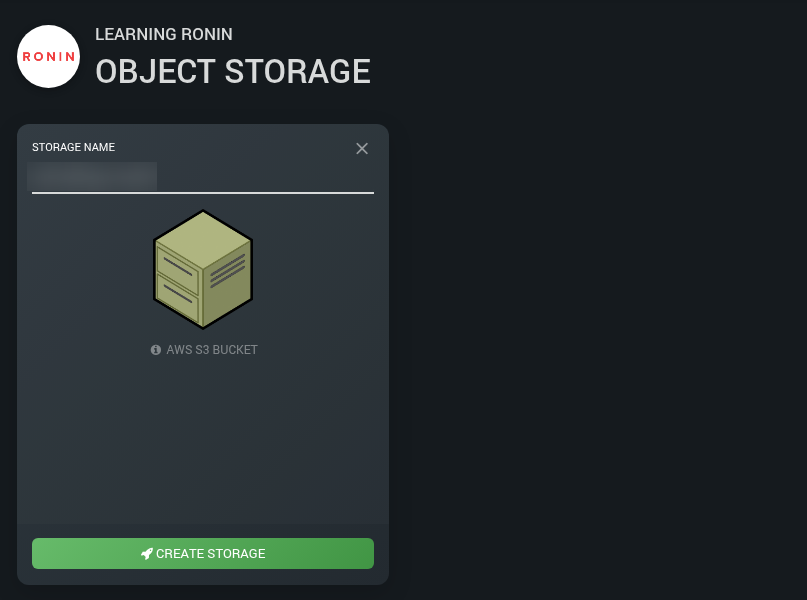
While the cluster builds, set up somewhere to put the results. Go to Object Storage, click NEW OBJECT STORE, give it a name and click CREATE STORAGE.
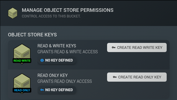
Next, make a key so the head node can write to the bucket. Click MANAGE PERMISSIONS on the bucket card, then CREATE READ WRITE KEY. Your browser downloads a small CSV file with the key. Keep it somewhere safe and never put it in a script or a shared folder.
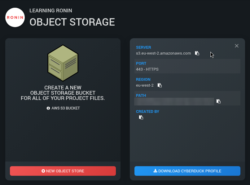
Finally, open the bucket's Connect Info from the three dots menu on its card and copy the PATH and REGION. You will need both in Step 8. The path looks like my-bucket.store.ronin.cloud.
Step 3: Connect and set up the environment
When your cluster is RUNNING, click OPEN IN RONIN LINK and open a terminal on the head node.
First, a few one-off preparations. The cluster's launch image does not include the AWS CLI or Python's venv module, so install them now:
sudo apt-get update && sudo apt-get install -y python3-venv unzip
# Install the AWS CLI
curl -s "https://awscli.amazonaws.com/awscli-exe-linux-x86_64.zip" -o awscliv2.zip
unzip -q awscliv2.zip && sudo ./aws/install
Now create a folder for the scripts on /data. The cluster shares /apps, /data and your home folder (/home) with every compute node. /tmp is local to each node. This tutorial keeps its scripts and the tile data on /data. Save the tutorial scripts in this folder.
mkdir -p /data/buildings-scripts
cd /data/buildings-scripts
This tutorial prints every script in full, in the Full scripts section at the end of this post. They are numbered in the order you use them:
- Script 1:
config.sh(Step 3) holds all the settings. - Script 2:
requirements.txt(Step 3) lists the Python packages. - Script 3:
00_setup_venv.sh(Step 3) builds the Python environment. - Script 4:
01_stage_data.sh(Step 4) downloads the data and splits it into chunks. - Script 5:
sn4_models.py(Step 5) defines the three building models. - Script 6:
detect_buildings.py(Step 5) finds the buildings in each tile. - Script 7:
02_detect_array.sbatch(Step 5) is the Slurm job array. - Script 8:
03_merge.sbatch(Step 7) is the Slurm merge job. - Script 9:
merge_results.py(Step 7) combines the results and checks them against the labels. - Script 10:
make_overlays.py(Step 7) draws the overlay images. - Script 11:
submit_all.sh(Step 5) submits the array and the merge job. - Script 12:
04_upload.sh(Step 8) uploads the results to your bucket.
Each listing is a single block that you copy and paste into your terminal while you are in /data/buildings-scripts. It creates the file for you, and for the shell scripts it also makes them executable. For this step, create Scripts 1, 2 and 3 now. You will create the rest as you reach the step that uses them.
config.sh (Script 1) is where everything is set. The defaults are what we used. The settings you are most likely to change are N_CHUNKS (how many array tasks, 100 for us, which is about 149 tiles per task), MAX_PARALLEL (how many may run at once), COLLECTS (which viewing angles to process) and DEST (your bucket path from Step 2).
Then build the Python environment on /apps, so every node uses the same one. 00_setup_venv.sh (Script 3) reads requirements.txt (Script 2) and installs CPU-only PyTorch, rasterio, Shapely and friends:
./00_setup_venv.sh
This should take around 38 seconds.
Step 4: Stage the data
Next, copy the tiles, SpaceNet's hand-drawn labels and the model weights from the public SpaceNet bucket to /data. No key is needed, because the bucket allows anonymous downloads. Create 01_stage_data.sh (Script 4 in the Full scripts section), then run it. You can run it in a second terminal while the venv builds.
./01_stage_data.sh
The script uses aws s3 sync --no-sign-request, so it is safe to run again if it is interrupted. At the end, it lists every tile and uses split to divide the list into 100 chunk files, one for each array task.
In our run, it staged 89.76 GB in 11 minutes 18 seconds (about 132 MB/s) and finished with:
Staged 14896 tiles into 100 chunks
Why stage at all, instead of reading straight from the bucket? Because 100 nodes reading from a shared drive is simple, fast and needs no credentials on the compute nodes. Object storage is great for keeping data, but it is usually better to copy files onto a drive before you process them.
Step 5: Detect buildings with a Slurm job array
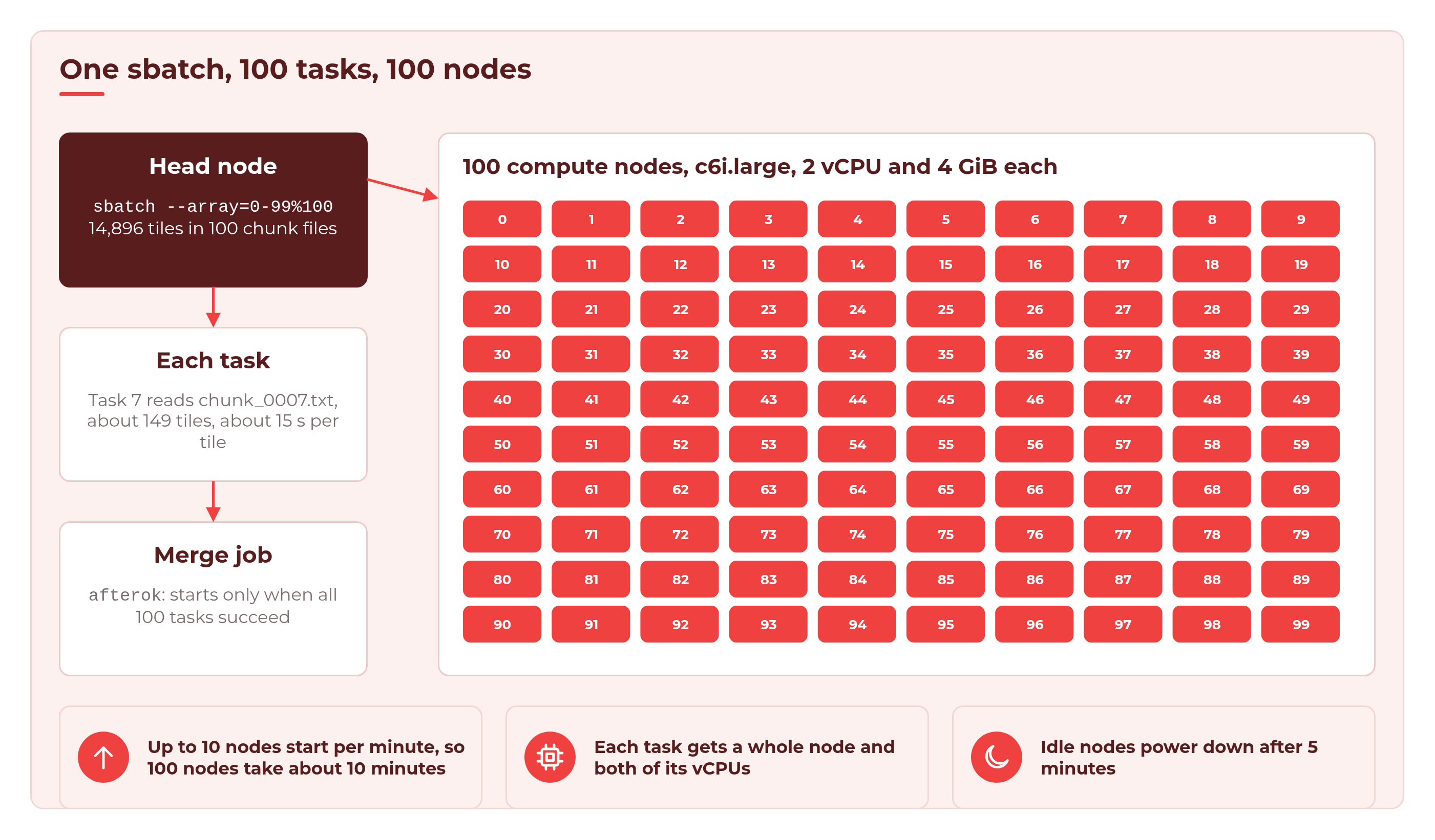
A job array lets you submit one script that runs many times, each with its own task ID. Task 7 reads chunk_0007.txt, task 42 reads chunk_0042.txt, and so on. With 100 tasks and Max nodes set to 100, every task gets its own node.
Create these scripts now, from the Full scripts section, in /data/buildings-scripts:
- Script 5:
sn4_models.pydefines the three U-Net models and loads their weights. - Script 6:
detect_buildings.pydoes the detection for one chunk of tiles. - Script 7:
02_detect_array.sbatchis the job array script. - Script 11:
submit_all.shsubmits the array and the merge job together.
submit_all.sh queues the merge job at the same moment as the array, so also create the three merge scripts now: Script 8 (03_merge.sbatch), Script 9 (merge_results.py) and Script 10 (make_overlays.py). We explain them in Step 7.
The top of 02_detect_array.sbatch tells Slurm what each task needs: --array=0-99%100 for 100 tasks with at most 100 running at once, --cpus-per-task=2 for a whole 2 vCPU node per task, --mem=3G and --time=01:00:00. Then each task works out its own chunk file from its task ID and runs detect_buildings.py on it, using the Python environment on /apps.
Each job gets the CPUs and memory it asks for. Without --cpus-per-task or --mem, a job gets 1 CPU and an even share of the node's memory for each CPU. Several jobs share a node until its CPUs or memory are used up. With hyperthreading on (the default), one Slurm CPU is one vCPU, so a 4 vCPU node can run four 1-CPU jobs at once. With hyperthreading off, each node offers one CPU per physical core. Slurm registers 90% of the node type's memory, so a 4 GiB c6i.large shows up as 3,686 MiB (about 3.6 GiB). That is why we ask for --mem=3G: our measured peak was about 1.9 GB per task (1,919 MB), which leaves plenty of room.
detect_buildings.py does the work on each tile. The three models each score every pixel, and the scores are averaged. A pixel counts as building when its averaged score is above 0.5. Pixels the models mark as building edges are dropped, so that buildings which touch are split apart. Each separate blob of at least 20 pixels (5 square metres) becomes one building, and is grown back out to its full outline.
For every tile, it writes a GeoJSON of outlines in longitude and latitude, plus one CSV row with the building count, total area, seconds taken and any error. An unreadable tile is recorded as an error and the task simply moves on, which is exactly what you want when cleaning a big dataset.
💡 Tip: Before you launch 100 nodes, test one tile on the head node. In our testing, one tile took about 10 seconds there and found 111 buildings. This runs the same detection code as an array task, on one tile:
source ./config.sh
grep nadir7_ "$DATA_ROOT/manifest.txt" | grep 739451_3732339 > /tmp/one_tile.txt
SLURM_CPUS_PER_TASK=2 "$VENV_DIR/bin/python" detect_buildings.py \
  /tmp/one_tile.txt "$MODEL_DIR" /tmp/one_tile_geojson /tmp/one_tile.csv
When you are ready, submit everything with one command. submit_all.sh submits the array, then a merge job that only starts if every array task succeeds (afterok):
$ ./submit_all.sh
Submitted detection array 1 (100 tasks, max 100 at once)
Submitted merge job 2 (waits for 1)
If you ever submit 02_detect_array.sbatch or 03_merge.sbatch by hand with sbatch, run mkdir -p /data/buildings/logs first. Both scripts write their log files there, and a job whose log folder is missing fails straight away. (submit_all.sh creates the folder for you.)
Now check on it with sinfo and squeue. Here is our cluster about five minutes in (a real capture from our run, with node names shortened and most of the queue left out):
$ sinfo
PARTITION AVAIL  TIMELIMIT  NODES  STATE NODELIST
main*        up   infinite     52  alloc ip-10-0-1-[10-61]
main*        up   infinite      5 alloc# ip-10-0-1-[62-66]
main*        up   infinite     43 alloc~ ip-10-0-1-[67-109]

$ squeue -u $USER
 JOBID PARTITION     NAME     USER ST  TIME  NODES NODELIST(REASON)
  1_57      main building   ubuntu CF  4:50      1 ip-10-0-1-67
  1_58      main building   ubuntu CF  4:50      1 ip-10-0-1-68
     2      main building   ubuntu PD  0:00      1 (Dependency)
  1_44      main building   ubuntu  R  0:09      1 ip-10-0-1-54
   1_0      main building   ubuntu  R  4:09      1 ip-10-0-1-10
   ...  (95 more tasks)
What this tells you:
allocnodes are up and working.alloc#nodes are powering up.alloc~nodes have a task waiting for them but are still powered off.- Tasks in state
CF(configuring) are waiting for their node to boot.Rmeans running. - Job 2, the merge, is
PD(pending) with the reason(Dependency). It waits for the whole array.
Why do the nodes arrive in waves? RONIN sets Slurm's ResumeRate to 10 nodes per minute. ResumeRate limits how many nodes Slurm powers up at once, so nodes launch at a steady rate. So 100 nodes take about 10 minutes to arrive, and the early tasks get a head start.
Step 6: Watch it scale in Grafana
This is the fun part. Every HPC Auto Scale Cluster comes with Grafana built in. In RONIN LINK, choose GRAFANA from the Default links to commonly used apps dropdown, click LINK and Grafana opens in your browser. There is no sign in. If you have not done this before, How to Use Grafana Dashboards on Your HPC Auto Scale Cluster walks you through it.
Here is our whole run, from submission to the last node powering down:
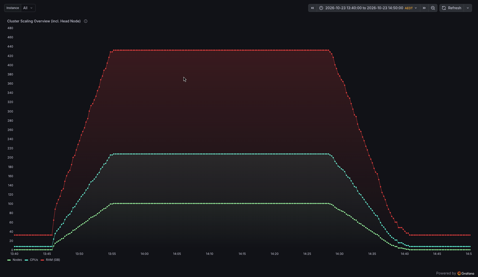
The shape is exactly what we hoped for:
- Ramp up (13:45 to 13:55 AEDT). About 10 nodes a minute. The first tasks were running within a minute of submitting, and all 100 were running after 10.5 minutes.
- Plateau (13:55 to about 14:23). 100 nodes, 200 compute vCPUs, every one of them busy.
- Tasks finish (14:23 to 14:35). Each task finishes after its own 149 tiles, so nodes go quiet one by one. The first finished at 14:22:59 and the last at 14:34:55.
- Power down (from about 14:28). About five minutes after a node goes idle, it powers down (Slurm's
SuspendTimeof 300 seconds). The last node was off at 14:41:39, 6 minutes 44 seconds after the last task finished.
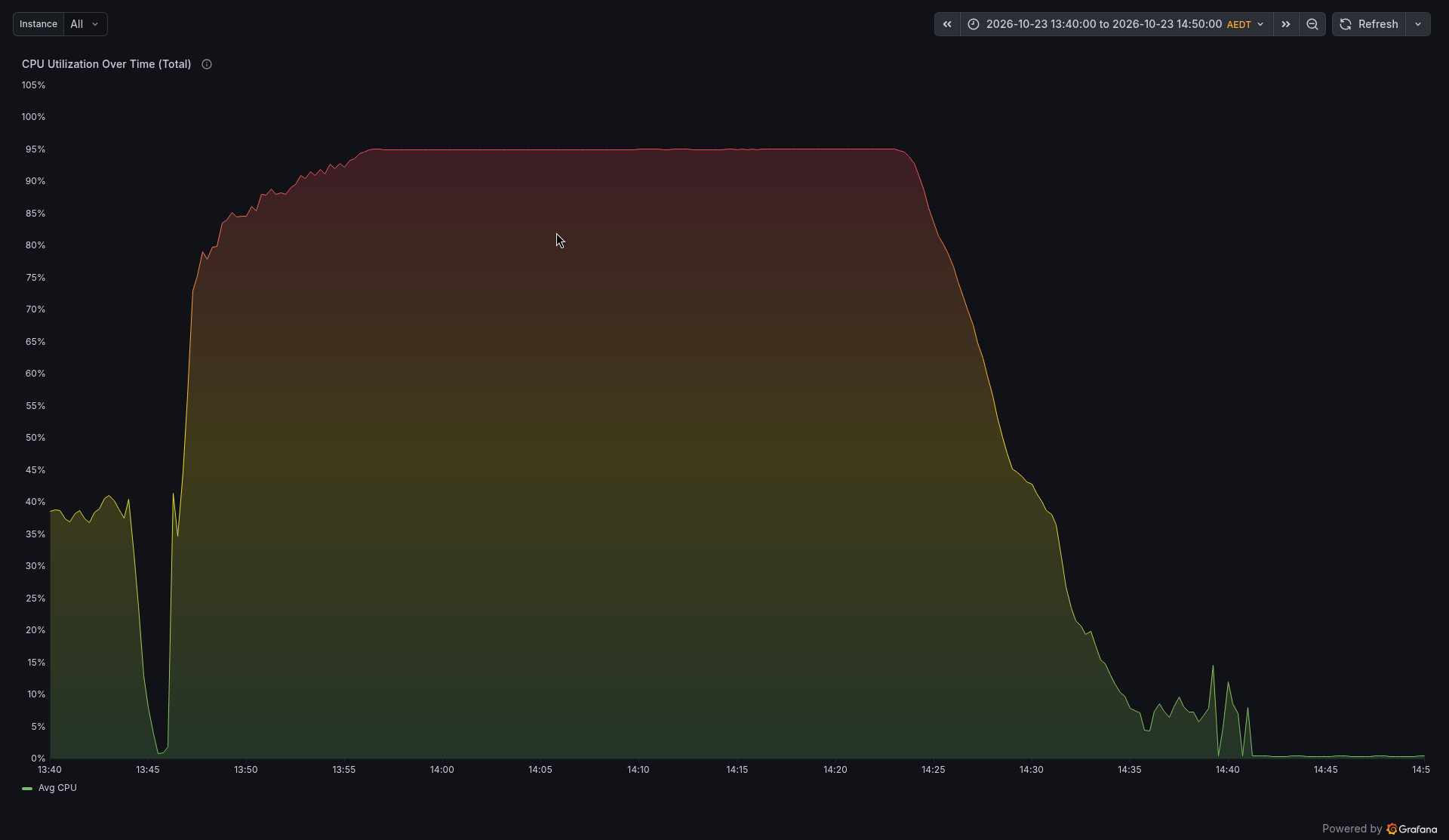
The CPU panel shows that the nodes were doing real work, not waiting around for data:
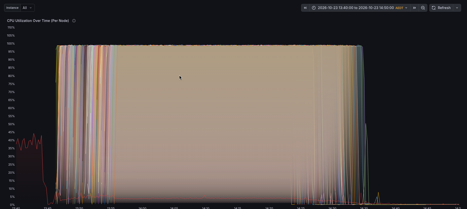
Switch to the per node CPU panel and you can see all 100 nodes, each one starting a little after the last:
The network panel tells the data story. Before 13:45 the head node is downloading tiles at about 130 MB/s. As nodes start, there is a burst while each one loads its Python environment and models. Then it settles to a steady stream while 100 nodes read their tiles from /data:
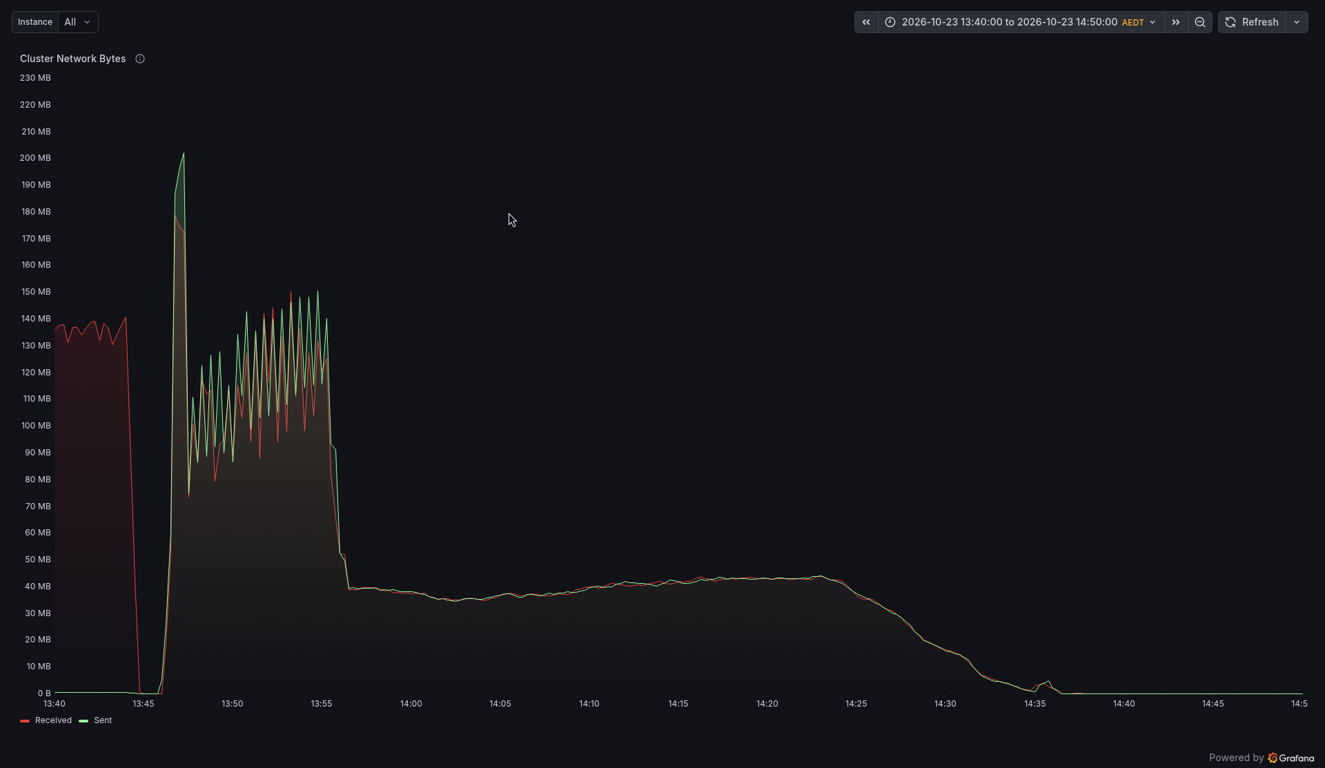
That steady part, about 40 MB/s, is a nice sanity check. 100 nodes each reading a 6 MB tile every 15 seconds comes to about 40 MB/s.
Want to see what the dashboard looked like in the middle of the run? Here it is at full power, with 100 nodes and the CPU gauge at 95%:
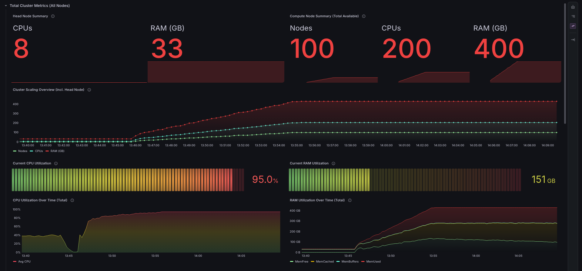
You can also pick any single node from the Instance menu to check on it:
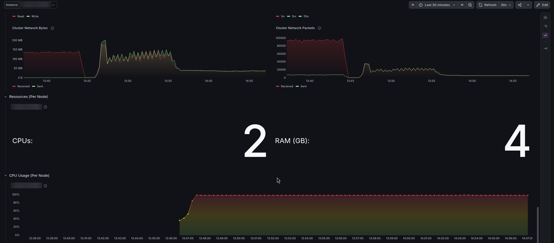
The RONIN cluster card tells the same story in one glance:
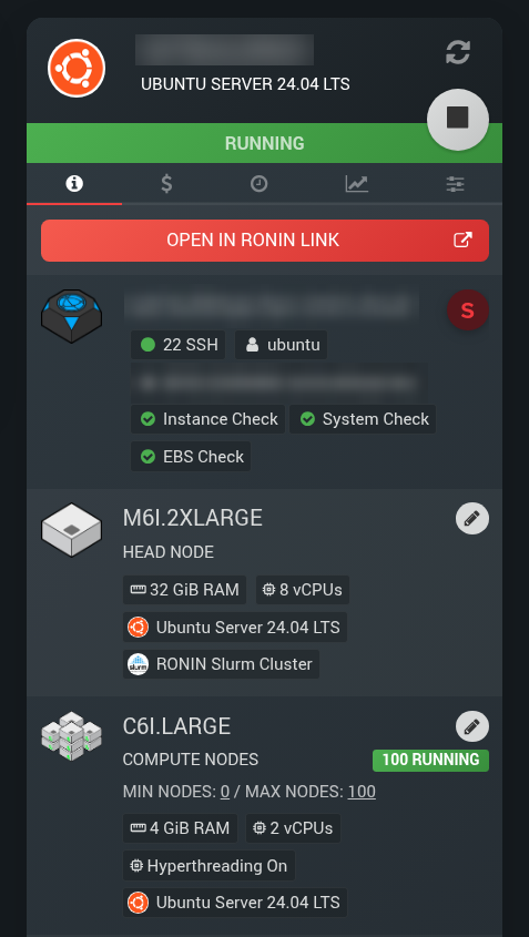
Then, a few minutes after each node's task ends, the nodes power down:
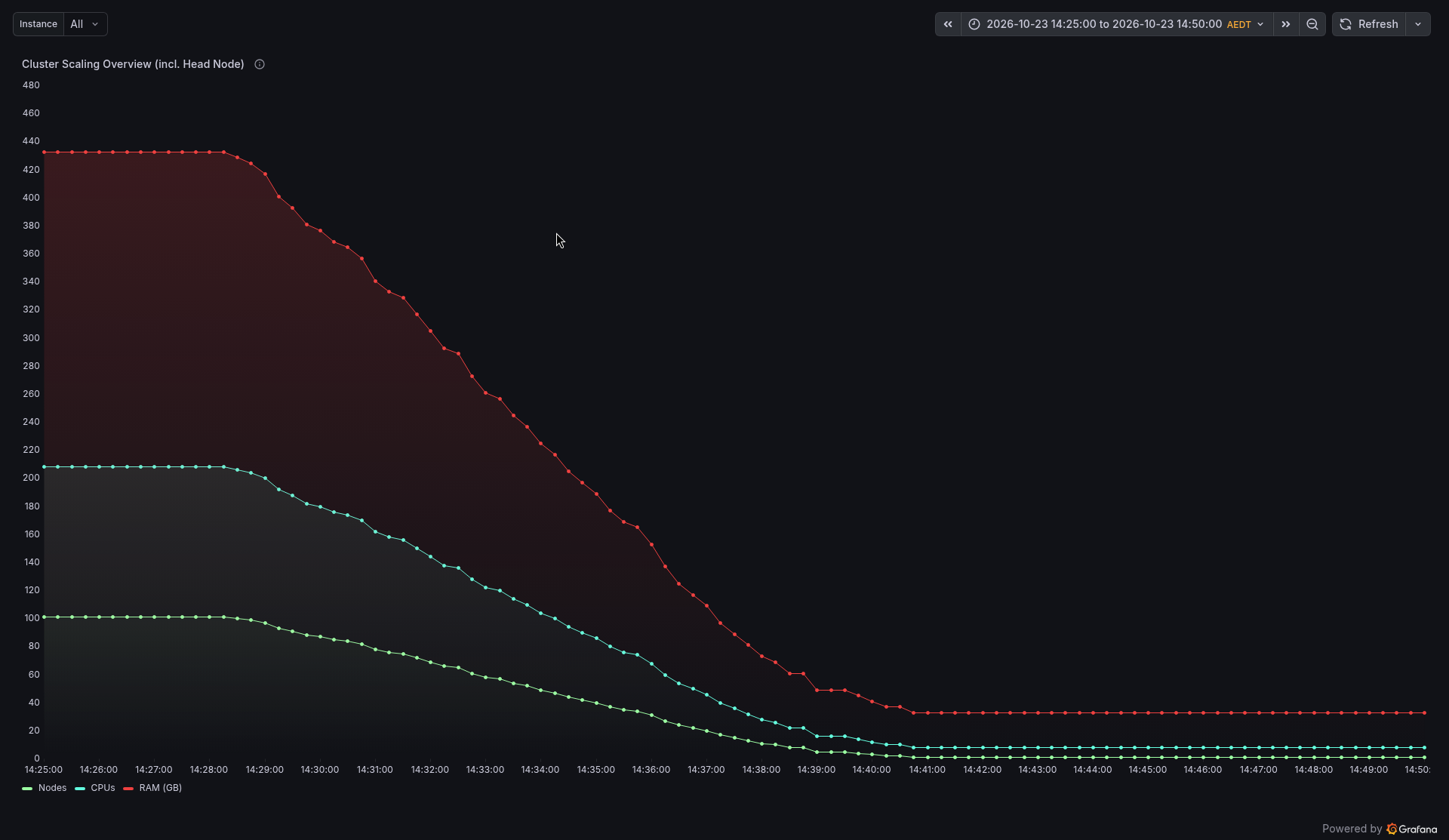
Here are the key times from our run (AEDT):
- 13:45:08 Array submitted
- 13:55:38 All 100 tasks running
- About 13:56 CPU plateau at about 95%
- 14:22:59 First task finished, plateau ends
- About 14:28 Idle nodes start powering down
- 14:34:55 Last task finished, merge starts
- 14:35 Merge finished, 33 seconds later
- 14:41:39 All compute nodes powered off
Every one of the 100 tasks ran on its own node and finished successfully. The fastest took 33 minutes 8 seconds, the slowest 41 minutes 53 seconds, and the median was 38 minutes 24 seconds. Each tile took about 15.4 seconds on one node, but with 100 nodes, the cluster got through about 5 tiles every second.
Step 7: Merge and check the quality
The moment the last task finished, Slurm started the merge job (03_merge.sbatch, Script 8). It runs merge_results.py (Script 9), which combines the 100 per task CSVs, counts SpaceNet's hand-drawn buildings for every tile, and writes the reports. Then it runs make_overlays.py (Script 10), which draws the detected outlines on the two busiest tiles, from the most overhead and the most oblique view. It took 33 seconds, and the merge printed:
           tiles_total: 14896
          tiles_failed: 0
              collects: 14
       buildings_found: 790221
    buildings_labelled: 917994
     building_area_km2: 257.47
 mean_seconds_per_tile: 15.39
   total_compute_hours: 63.7
No broken tiles, and 790,221 detections against 917,994 labels (65,571 hand-drawn outlines, one set per view). That is 86% as many detections as labels overall. (Each of the roughly 65,600 unique buildings can be counted up to 14 times, once per view, and the area adds up all 14 views in the same way.)
The more interesting result is in per_collect.csv, which splits the count by viewing angle:
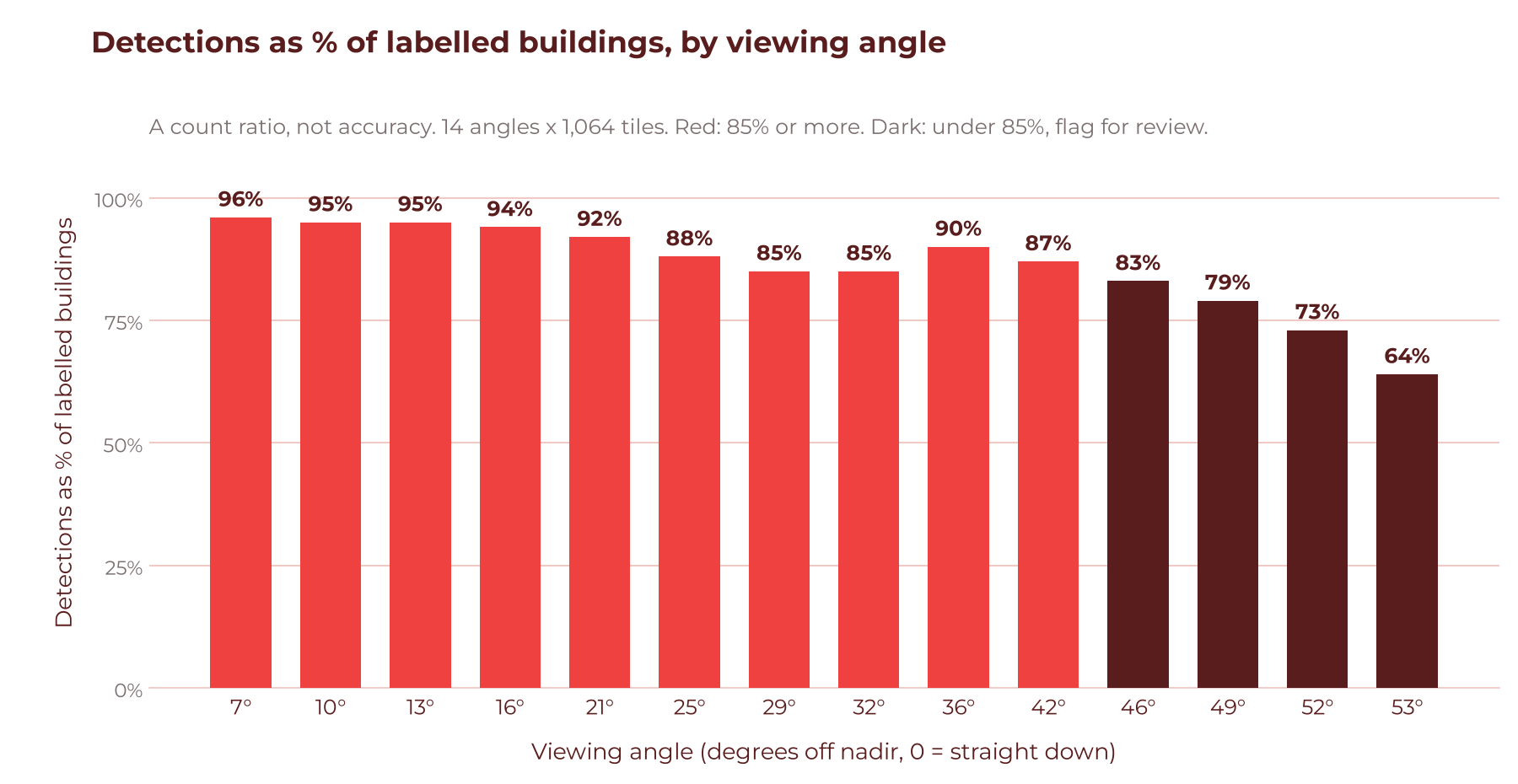
Looking almost straight down, the models found 96% as many buildings as were labelled (a count ratio, not accuracy). At 53 degrees, they found only 64% as many. That makes sense: at steep angles, buildings lean over, hide behind each other and cast long shadows. A count ratio does not check that each outline lands on the right building; SpaceNet itself scores models with F1 at an IoU (overlap) of 0.5, matching each outline to a labelled one.
This is exactly the kind of thing you want to know before you train a model. Put the two views side by side and you can see it straight away:
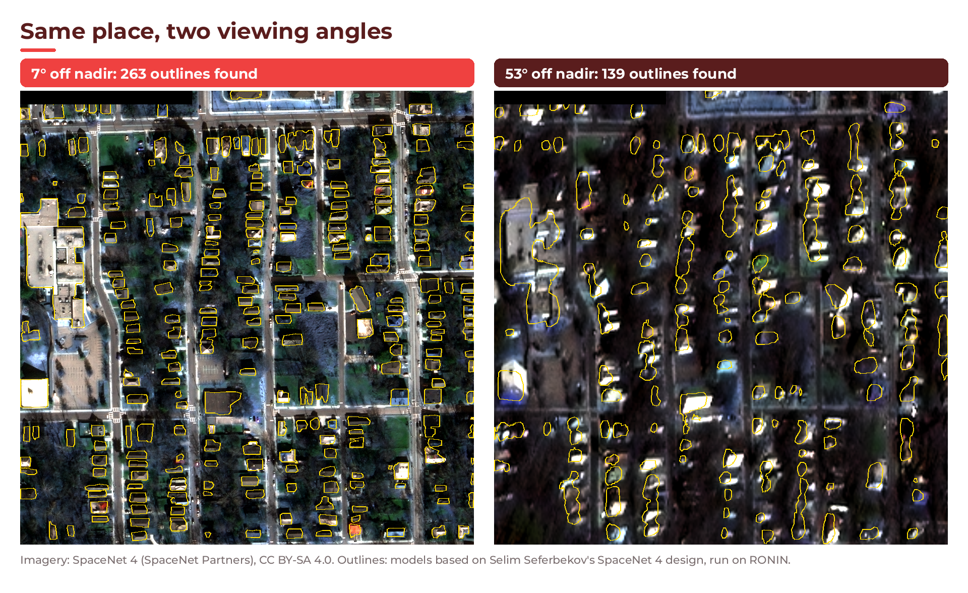
A few quick quality checks you can run on all_tiles.csv:
python3 - <<'PY'
import csv
rows = list(csv.DictReader(open("/data/buildings/reports/all_tiles.csv")))
errors = [r for r in rows if r["error"]]
empty = [r for r in rows if not r["error"] and int(r["buildings"]) == 0]
print(len(rows), "tiles,", len(errors), "errors,", len(empty), "with no buildings")
PY
In our run, that printed 14896 tiles, 0 errors, 625 with no buildings. That is 4.2% of tiles worth a look before training: some will be genuinely empty (fields, car parks, water), and some may be detections that went wrong.
💡 Tip: One honest caveat. These pretrained models were trained on SpaceNet 4 Atlanta imagery, which is the data we process here, so results here may look better than they would on imagery the models have never seen. That is fine for showing the workflow. For your own data, check a held-out sample by hand.
Step 8: Upload the results to your RONIN bucket
Now save the results. The upload runs on the head node, where you set up your bucket key with aws configure.
Create 04_upload.sh (Script 12 in the Full scripts section) if you have not already. Then add your bucket key as an AWS CLI profile. Paste the access key ID and secret from the CSV you downloaded in Step 2, and use the region from Connect Info:
aws configure --profile ronin-bucket
export AWS_PROFILE=ronin-bucket
export DEST=s3://my-bucket.store.ronin.cloud/spacenet4-buildings
Do a dry run first, then the real upload:
DRY_RUN=1 ./04_upload.sh
./04_upload.sh
The script first checks for a MERGE_DONE file and stops with a message if the merge has not finished. Otherwise it runs two aws s3 sync commands, one for the GeoJSONs and one for the reports. The 89 GB of raw tiles stay behind on /data. In our run, it uploaded 14,905 objects, 412.1 MB, in 47 seconds:
$ aws s3 ls --recursive --summarize $DEST/ | tail -2
Total Objects: 14905
   Total Size: 412125103
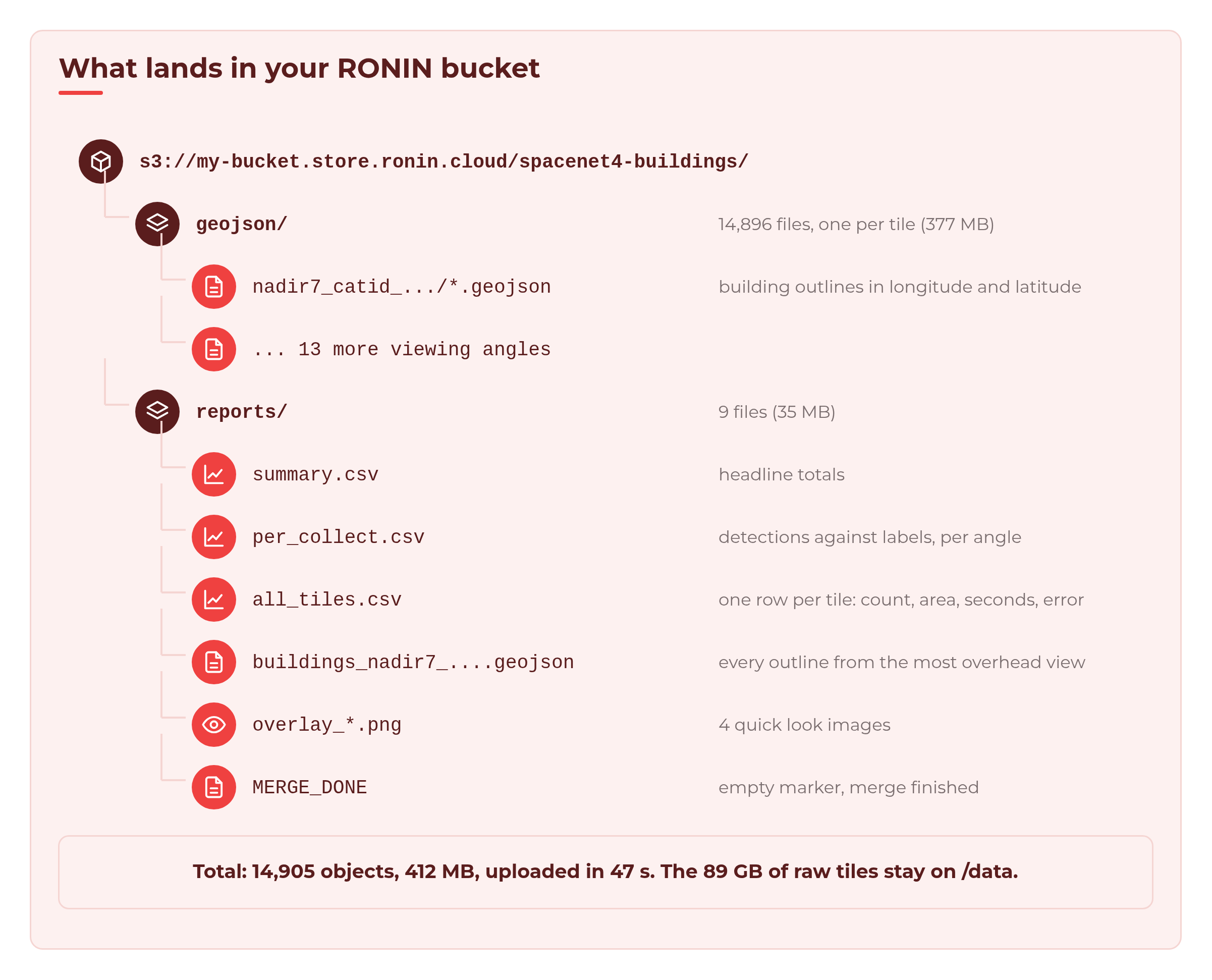
💡 Tip: 14,896 small files means 14,896 upload requests. For a much bigger dataset, run
PACK=1 ./04_upload.shto upload one archive instead.
Back in RONIN, your bucket card shows the READ WRITE key. The size on the card is not live. It can take up to 48 hours to update, so do not worry if it still says EMPTY for a while.
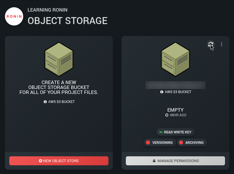
aws s3 ls to check straight away.Step 9: Clean up
Make sure the queue is empty first (squeue -u $USER). Stopping a cluster ends any running jobs and clears the queue.
You have three choices:
- Keep it. With Min nodes at 0, the compute nodes are already off. Only the head node and drives keep costing money.
- Stop it from the cluster card, and start it again when you need it.
- Terminate it when you are completely done. On the cluster card, open the Actions tab and click TERMINATE CLUSTER. This deletes the cluster and its drives, including the 90 GB of tiles on /data, unless you have snapshotted the drives or nominated a drive to keep, as with single machines, so make sure your results are safely in the bucket first.

Do not forget the bucket key. If you no longer need it, delete or replace it under MANAGE PERMISSIONS.
What it cost
The cluster's Cost tab shows what you are spending right now. Here it is at the peak, with all 100 nodes running:
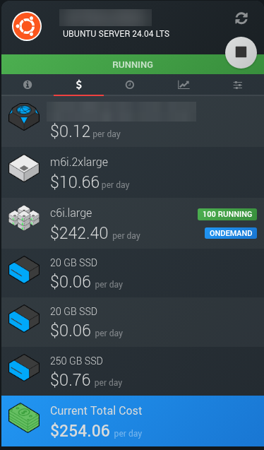
But it only runs at that rate for about half an hour. Here is how a run like ours adds up (USD, eu-west-2 London on demand prices, approximate):
- Compute nodes: about $7.65. About 76 node-hours of c6i.large at about $0.10 an hour, including start-up and each node's 5 idle minutes.
- Head node: about $0.67. About 1.5 hours of m6i.2xlarge at about $0.44 an hour, covering setup, staging, the run and the upload.
- Drives and bucket: a few cents. A few hours of 290 GB of drives, plus 412 MB in the bucket.
- Total: about $8.
Of those 76 node-hours, 63.7 were spent actually detecting buildings. The rest was nodes starting up and waiting their 5 idle minutes before powering down. That is the price of never having to remember to turn anything off.
Compare that with one 2 vCPU machine working through all 14,896 tiles one after another: 63.7 hours, or about 2.6 days. Same work, same type of node, roughly the same cost, but you get your answer the same afternoon instead of next week.
Next steps: getting ready for AI training
You now have a clean, checked set of building labels for 14,896 tiles. From here you could:
- Use the outlines as training labels for your own building detector, or as a second opinion on existing labels.
- Filter your dataset. Drop or review tiles with errors, tiles with no buildings, or whole viewing angles where the detection count ratio falls below a threshold you choose (for example, under 85%).
- Look for label problems. Tiles where the models and the hand-drawn labels disagree a lot are worth checking. Sometimes the labels are wrong, not the model.
- Go bigger. Change
COLLECTSinconfig.shto process all 27 angles (28,728 tiles, about 168 GB), or point the scripts at your own imagery. The pattern stays the same: stage, array, merge, upload. - Try a different node type. See Bigger, Smaller, More or Fewer: Changing Compute Nodes in an HPC Auto Scale Cluster.
Troubleshooting
Fewer nodes start than I expected. Check Max nodes, and ask your RONIN admin to check your vCPU quota on the Service Quota screen. 100 x 2 vCPU nodes plus the head node needs about 208 vCPUs.
My tasks are stuck in CF or PD. CF means the node is still booting; with Min nodes at 0, expect up to about 10 minutes for all 100 nodes. PD with (Dependency) on the merge job is normal until the array finishes.
The merge job never starts. If any array task fails, the merge job stays pending with the reason DependencyNeverSatisfied, because it only runs when every task succeeds. Check the task logs in /data/buildings/logs, fix the problem, then cancel the stuck merge job with scancel and its job ID (from squeue -u $USER) before you submit again.
Tasks fail with "No such file or directory". Your scripts may be in a folder only the head node can see, such as /tmp. Move them to /data or your home folder, which every compute node can see.
The upload says Access Denied. Check that you used the READ WRITE key (not read only), the region from Connect Info, and that AWS_PROFILE is set in the terminal you are using.
Wrapping up
In under an hour, a cluster that cost only its head node and drives while idle grew to 100 nodes, traced 790,221 building outlines in 14,896 satellite tiles, checked them against hand-drawn labels, and then quietly switched itself off. The results are waiting in your bucket for the fun part: training.
For everything else that is new in HPC Auto Scale Clusters, see Meet the New HPC Auto Scale Clusters.
Full scripts
Here is every script this tutorial uses, printed in full and in the order you use them. Save all of them in /data/buildings-scripts (the folder from Step 3). Each listing is one block you can copy and paste into your terminal. The first line creates the file and the line EOF ends it. Where a script needs to be run directly, the last line makes it executable. If you prefer an editor, run nano with the file name instead, paste only the lines between the first line and EOF, then save.
The only value you need to change is the bucket path in config.sh, and you can also set that with export DEST= when you upload in Step 8.
Script 1: config.sh
Holds every path and setting in one place. Every other script reads it, so this is the file you edit to change the number of tasks, the angles you process or where the results go. Used in Step 3.
cat > config.sh <<'EOF'
#!/usr/bin/env bash
# shellcheck disable=SC2034  # variables are used by the scripts that source this file
# config.sh - one place to edit paths and settings. Every other script sources this.
# Values can be overridden from the environment, e.g. N_CHUNKS=4 ./01_stage_data.sh

# Shared cluster storage (visible to the head node and every compute node)
DATA_ROOT="${DATA_ROOT:-/data/buildings}"           # all data lives under here
APPS_ROOT="${APPS_ROOT:-/apps}"                     # shared software
VENV_DIR="${VENV_DIR:-$APPS_ROOT/venvs/buildings}"  # Python venv used by every job

RAW_DIR="$DATA_ROOT/raw"           # satellite tiles, one folder per collect
LABEL_DIR="$DATA_ROOT/labels"      # SpaceNet's hand-drawn building outlines (for comparison)
MODEL_DIR="$DATA_ROOT/models"      # pretrained model weights
CHUNK_DIR="$DATA_ROOT/chunks"      # one text file of tile paths per array task
OUT_DIR="$DATA_ROOT/geojson"       # one GeoJSON of building outlines per tile
RESULTS_DIR="$DATA_ROOT/results"   # one CSV per array task
REPORT_DIR="$DATA_ROOT/reports"    # merged CSVs and overlay PNGs
LOG_DIR="$DATA_ROOT/logs"          # Slurm stdout/stderr

# Open data: SpaceNet 4 (Atlanta), public bucket, no AWS account needed (us-east-1)
SRC="s3://spacenet-dataset/spacenet/SN4_buildings/train/AOI_6_Atlanta"
MODEL_SRC="s3://spacenet-dataset/spacenet-model-weights/spacenet-4"
MODELS="${MODELS:-densenet121unet densenet161unet resnet34unet}"  # averaged together

# The same 1,064 tile locations were photographed 27 times from different angles
# ("nadir7" = 7 degrees off vertical). We use every second angle: 14 x 1,064 =
# 14,896 tiles, ~89 GB. Fewer collects = less work.
COLLECTS="${COLLECTS:-nadir7_catid_1030010003D22F00 nadir10_catid_1030010003993E00
nadir13_catid_1030010002B7D800 nadir16_catid_1030010002649200 nadir21_catid_1030010003127500
nadir25_catid_103001000307D800 nadir29_catid_1030010003315300 nadir32_catid_103001000392F600
nadir36_catid_1030010003895500 nadir42_catid_10300100035D1B00 nadir46_catid_1030010003713C00
nadir49_catid_1030010003492700 nadir52_catid_1030010003BDDC00 nadir53_catid_1030010003CD4300}"
SAMPLE_TILES="${SAMPLE_TILES:-}"   # testing: only these tile locations, e.g. "739451_3732339"

# How many array tasks to split the work into, and how many may run at once
N_CHUNKS="${N_CHUNKS:-100}"         # 14,896 tiles / 100 = ~149 tiles per task
MAX_PARALLEL="${MAX_PARALLEL:-100}" # ~100 compute nodes x 2 vCPUs

# Where results go at the end (used by 04_upload.sh on the head node).
# RONIN buckets are ordinary S3 buckets. Copy your bucket path from
# RONIN > Object Storage > (your bucket) > Connect Info; it looks like
# my-bucket.store.ronin.cloud. A local folder path also works, for testing.
DEST="${DEST:-s3://my-bucket.store.ronin.cloud/spacenet4-buildings}"
EOF
chmod +x config.sh
Script 2: requirements.txt
Lists the Python packages the environment needs, including the CPU-only build of PyTorch. Used in Step 3.
cat > requirements.txt <<'EOF'
# CPU-only PyTorch wheels (much smaller than the default CUDA build)
--extra-index-url https://download.pytorch.org/whl/cpu
torch>=2.2
torchvision>=0.17
numpy>=1.26
scipy>=1.11
rasterio>=1.3
shapely>=2.0
pillow>=10.0
EOF
Script 3: 00_setup_venv.sh
Builds one shared Python virtual environment on /apps and installs the packages from requirements.txt. Used in Step 3.
cat > 00_setup_venv.sh <<'EOF'
#!/usr/bin/env bash
# 00_setup_venv.sh - create a Python virtual environment on shared storage (/apps)
# Run once on the head node; every compute node then uses the same venv.
# Downloads ~250 MB of wheels (CPU-only PyTorch, rasterio, ...).
set -euo pipefail
source "$(dirname "$0")/config.sh"

mkdir -p "$(dirname "$VENV_DIR")"
python3 -m venv "$VENV_DIR"                  # needs the python3-venv package on Ubuntu
"$VENV_DIR/bin/pip" install --upgrade pip
"$VENV_DIR/bin/pip" install -r "$(dirname "$0")/requirements.txt"

"$VENV_DIR/bin/python" -c 'import torch, rasterio; print("torch", torch.__version__, "| rasterio", rasterio.__version__)'
echo "Venv ready: $VENV_DIR"
EOF
chmod +x 00_setup_venv.sh
Script 4: 01_stage_data.sh
Copies the tiles, SpaceNet labels and model weights from the public SpaceNet bucket to /data, then splits the tile list into one chunk file per array task. Used in Step 4.
cat > 01_stage_data.sh <<'EOF'
#!/usr/bin/env bash
# 01_stage_data.sh - copy the SpaceNet 4 tiles, labels and model weights to /data,
# then split the tile list into one chunk per array task.
# Run on the head node. Needs the AWS CLI, but no key: the SpaceNet bucket is public
# (--no-sign-request). Safe to re-run: `aws s3 sync` skips files you already have.
set -euo pipefail
source "$(dirname "$0")/config.sh"
mkdir -p "$RAW_DIR" "$LABEL_DIR" "$MODEL_DIR" "$CHUNK_DIR"
S3=(aws s3)

# 1. Model weights (~350 MB for the three models)
for m in $MODELS; do
  "${S3[@]}" cp "$MODEL_SRC/selimsef_spacenet4_${m}_solaris_weights.pth" "$MODEL_DIR/$m.pth" --only-show-errors --no-sign-request
done

# 2. Hand-drawn building outlines for the 1,064 locations (~120 MB, used only for comparison)
"${S3[@]}" sync "$SRC/geojson_buildings/" "$LABEL_DIR/" --only-show-errors --no-sign-request

# 3. The 4-band images (red, green, blue, near-infrared; 900 x 900 pixels, resampled to 0.5 m per pixel), per collect
for c in $COLLECTS; do
  echo "Downloading $c"
  if [[ -n "$SAMPLE_TILES" ]]; then  # test mode: only a few tile locations
    for t in $SAMPLE_TILES; do
      f="SN4_buildings_train_AOI_6_Atlanta_${c}_PS-RGBNIR_$t.tif"
      "${S3[@]}" cp "$SRC/$c/PS-RGBNIR/$f" "$RAW_DIR/$c/$f" --only-show-errors --no-sign-request
    done
  else
    "${S3[@]}" sync "$SRC/$c/PS-RGBNIR/" "$RAW_DIR/$c/" --only-show-errors --no-sign-request
  fi
done

# 4. List every tile and split the list into N_CHUNKS files: chunk_0000.txt, chunk_0001.txt, ...
find "$RAW_DIR" -name "*.tif" | sort > "$DATA_ROOT/manifest.txt"
rm -f "$CHUNK_DIR"/chunk_*.txt
split -n "r/$N_CHUNKS" -d -a 4 --additional-suffix=.txt "$DATA_ROOT/manifest.txt" "$CHUNK_DIR/chunk_"
echo "Staged $(wc -l < "$DATA_ROOT/manifest.txt") tiles into $(find "$CHUNK_DIR" -name 'chunk_*.txt' | wc -l) chunks"
EOF
chmod +x 01_stage_data.sh
Script 5: sn4_models.py
Defines the three U-Net building models and loads their published weights. It is a short re-write of model code from Solaris (Apache 2.0, CosmiQ Works). Used in Step 5.
cat > sn4_models.py <<'EOF'
"""The three pretrained SpaceNet 4 building models.

This is a short re-write of the model code in the Solaris library
(https://github.com/CosmiQ/solaris, solaris/nets/zoo/selim_sef_sn4.py,
Apache License 2.0). The encoders come from torchvision. The layer names match
the published weight files, so the weights load as they are.

Each model takes a 4-band image (the PS-RGBNIR bands, in file order) and
returns 3 channels: building footprint, building edge and the contact
area between buildings.
"""
import torch
from torch import nn
from torchvision.models import densenet121, densenet161, resnet34


def conv_relu(c_in, c_out):
    return nn.Sequential(nn.Conv2d(c_in, c_out, 3, padding=1), nn.ReLU(inplace=True))


class Up(nn.Module):  # 2x upsample, then a 3x3 conv
    def __init__(self, c_in, c_out):
        super().__init__()
        self.layer = nn.Sequential(nn.Upsample(scale_factor=2),
                                   nn.Conv2d(c_in, c_out, 3, padding=1), nn.ReLU(inplace=True))

    def forward(self, x):
        return self.layer(x)


class Merge(nn.Module):  # join decoder and skip connection
    def __init__(self, c_in, c_out):
        super().__init__()
        self.seq = conv_relu(c_in, c_out)

    def forward(self, dec, enc):
        return self.seq(torch.cat([dec, enc], dim=1))


class UNet(nn.Module):
    def __init__(self, stages, filters, decoder_filters):
        super().__init__()
        self.encoder_stages = nn.ModuleList(stages)
        n = len(decoder_filters)
        self.bottlenecks = nn.ModuleList(
            Merge(filters[-i - 2] + f, f) for i, f in enumerate(reversed(decoder_filters)))
        self.decoder_stages = nn.ModuleList(
            Up(filters[i + 1] if i + 1 == n else decoder_filters[i + 1], decoder_filters[i])
            for i in range(n))
        last = 64
        self.last_upsample = Up(decoder_filters[0], last)
        self.final = nn.Sequential(nn.Conv2d(last, 3, 1))

    def forward(self, x):
        skips = []
        for stage in self.encoder_stages:
            x = stage(x)
            skips.append(x)
        for i, merge in enumerate(self.bottlenecks):
            x = merge(self.decoder_stages[-(i + 1)](x), skips[-(i + 2)])
        return self.final(self.last_upsample(x))


def _densenet(make, filters, decoder_filters):
    f = make(weights=None).features
    f.conv0 = nn.Conv2d(4, f.conv0.out_channels, 7, stride=2, padding=3, bias=False)
    stages = [nn.Sequential(f.conv0, f.norm0, f.relu0),
              nn.Sequential(f.pool0, f.denseblock1),
              nn.Sequential(f.transition1, f.denseblock2),
              nn.Sequential(f.transition2, f.denseblock3),
              nn.Sequential(f.transition3, f.denseblock4, f.norm5, nn.ReLU())]
    return UNet(stages, filters, decoder_filters)


def _resnet34():
    r = resnet34(weights=None)
    r.conv1 = nn.Conv2d(4, 64, 7, stride=2, padding=3, bias=False)
    stages = [nn.Sequential(r.conv1, r.bn1, r.relu),
              nn.Sequential(r.maxpool, r.layer1), r.layer2, r.layer3, r.layer4]
    return UNet(stages, [64, 64, 128, 256, 512], [64, 128, 256, 512])


BUILDERS = {
    "densenet121unet": lambda: _densenet(densenet121, [64, 256, 512, 1024, 1024], [64, 128, 256, 256]),
    "densenet161unet": lambda: _densenet(densenet161, [96, 384, 768, 2112, 2208], [64, 128, 256, 256]),
    "resnet34unet": _resnet34,
}


def load_model(name, weights_file):
    model = BUILDERS[name]()
    model.load_state_dict(torch.load(weights_file, map_location="cpu"))
    return model.eval()
EOF
Script 6: detect_buildings.py
Finds the buildings in every tile of one chunk and writes a GeoJSON file per tile and a results CSV for the chunk. Used in Step 5.
cat > detect_buildings.py <<'EOF'
#!/usr/bin/env python3
"""Find buildings in a list of satellite tiles. One Slurm array task runs this once.

Usage: detect_buildings.py CHUNK_FILE MODEL_DIR OUT_DIR RESULTS_CSV

For each tile, three pretrained U-Nets predict which pixels are building, and we
average them. Each separate blob of building pixels counts as one building and
becomes a polygon. Writes one GeoJSON per tile (OUT_DIR/<collect>/<tile>.geojson)
and one CSV row per tile.
"""
import csv
import json
import os
import resource
import sys
import time
from pathlib import Path

import numpy as np
import rasterio
import torch
import torch.nn.functional as F
from rasterio.features import shapes
from rasterio.warp import transform_geom
from scipy import ndimage
from shapely.geometry import mapping, shape

from sn4_models import load_model

MODELS = os.environ.get("MODELS", "densenet121unet densenet161unet resnet34unet").split()
# Per-band mean and spread used when the models were trained (Solaris config files)
MEAN = np.array([0.006479, 0.009328, 0.01123, 0.02082]) * 65535
STD = np.array([0.004986, 0.004964, 0.004950, 0.004878]) * 65535
THRESHOLD = 0.5      # a pixel is "building" if the averaged score is above this
MIN_PIXELS = 20      # ignore blobs under 20 pixels (5 m^2 at 0.5 m per pixel)
GROW_PIXELS = 3      # how far a building's core may grow back out to its full outline
SIMPLIFY_M = 0.5     # smooth the pixel staircase on polygon edges (metres)

FIELDS = ["tile", "collect", "nadir_deg", "buildings", "building_area_m2", "seconds", "error"]


def predict(models, img):
    """Average building/edge scores from all models. img is (4, H, W) uint16."""
    x = (img.transpose(1, 2, 0) - MEAN) / STD
    x = torch.from_numpy(x.transpose(2, 0, 1)[None].astype(np.float32))
    h, w = x.shape[2:]
    ph, pw = (-h) % 32, (-w) % 32  # the U-Nets need sizes divisible by 32
    x = F.pad(x, (pw // 2, pw - pw // 2, ph // 2, ph - ph // 2), mode="reflect")
    with torch.inference_mode():
        y = torch.stack([torch.sigmoid(m(x)) for m in models]).mean(0)[0]
    return y[:, ph // 2:ph // 2 + h, pw // 2:pw // 2 + w].numpy()


def find_buildings(scores, valid):
    """Turn scores into a label image: 0 = background, 1..n = building n."""
    footprint = (scores[0] > THRESHOLD) & valid
    core = footprint & (scores[1] < THRESHOLD)  # drop edge pixels so touching buildings split
    labels, n = ndimage.label(core)
    sizes = ndimage.sum(core, labels, range(1, n + 1))
    labels[np.isin(labels, np.flatnonzero(sizes < MIN_PIXELS) + 1)] = 0
    # grow each core back out over nearby footprint pixels
    dist, (iy, ix) = ndimage.distance_transform_edt(labels == 0, return_indices=True)
    grown = labels[iy, ix]
    grown[~footprint | (dist > GROW_PIXELS)] = 0
    return grown


def process(path, models, out_dir):
    collect = path.parent.name
    with rasterio.open(path) as src:
        img, transform, crs = src.read(), src.transform, src.crs
    if img.shape[0] != 4:
        raise ValueError(f"expected 4 bands, got {img.shape[0]}")
    labels = find_buildings(predict(models, img), valid=img.any(axis=0))

    features, area = [], 0.0
    for geom, _ in shapes(labels.astype(np.int32), mask=labels > 0, transform=transform):
        poly = shape(geom).simplify(SIMPLIFY_M)          # metres (UTM)
        area += poly.area
        features.append({"type": "Feature",
                         "properties": {"area_m2": round(poly.area, 1)},
                         "geometry": transform_geom(crs, "EPSG:4326", mapping(poly), precision=7)})
    out = out_dir / collect / (path.stem + ".geojson")
    out.parent.mkdir(parents=True, exist_ok=True)
    out.write_text(json.dumps({"type": "FeatureCollection", "features": features}))
    return collect, len(features), round(area, 1)


def main():
    chunk, model_dir, out_dir, results_csv = sys.argv[1:5]
    torch.set_num_threads(int(os.environ.get("SLURM_CPUS_PER_TASK", "2")))
    models = [load_model(m, Path(model_dir) / f"{m}.pth") for m in MODELS]
    paths = [Path(p) for p in Path(chunk).read_text().split()]
    Path(results_csv).parent.mkdir(parents=True, exist_ok=True)

    start = time.time()
    with open(results_csv, "w", newline="") as f:
        writer = csv.DictWriter(f, FIELDS)
        writer.writeheader()
        for i, path in enumerate(paths, 1):
            t0 = time.time()
            row = {"tile": path.name, "collect": path.parent.name,
                   "nadir_deg": path.parent.name.split("_")[0].removeprefix("nadir")}
            try:
                _, row["buildings"], row["building_area_m2"] = process(path, models, Path(out_dir))
            except Exception as e:  # a broken file shouldn't stop the other tiles
                row["error"] = f"{type(e).__name__}: {e}"[:200]
            row["seconds"] = round(time.time() - t0, 2)
            writer.writerow(row)
            f.flush()  # rows survive even if the job is killed part-way
            print(f"[{i}/{len(paths)}] {path.name}: {row.get('buildings', 'ERROR')} buildings, "
                  f"{row['seconds']} s", flush=True)

    peak_mb = resource.getrusage(resource.RUSAGE_SELF).ru_maxrss / 1024
    print(f"Done: {len(paths)} tiles in {time.time() - start:.0f} s, "
          f"{len(MODELS)} models, peak memory {peak_mb:.0f} MB")


if __name__ == "__main__":
    main()
EOF
Script 7: 02_detect_array.sbatch
The Slurm job array script: each task runs detect_buildings.py on its own chunk, on its own node. Used in Step 5.
cat > 02_detect_array.sbatch <<'EOF'
#!/usr/bin/env bash
# 02_detect_array.sbatch - one Slurm array task finds buildings in one chunk of tiles.
# Submit with ./submit_all.sh (it sets --array to match the number of chunks),
# or by hand:  sbatch --array=0-99%100 02_detect_array.sbatch
#SBATCH --job-name=buildings
#SBATCH --array=0-99%100           # 100 tasks, at most 100 running at once
#SBATCH --nodes=1
#SBATCH --ntasks=1
#SBATCH --cpus-per-task=2          # a whole 2 vCPU node per task
#SBATCH --mem=3G                   # measured peak ~1.9 GB (1,919 MB); a c6i.large offers 3,686 MiB (~3.6 GiB)
#SBATCH --time=01:00:00            # measured 33 to 42 min per task; generous safety margin
#SBATCH --output=/data/buildings/logs/%x_%A_%a.out   # %A = job ID, %a = task ID
set -euo pipefail
# Slurm copies the script to a spool dir, so find config.sh via the submit directory
HERE="${SLURM_SUBMIT_DIR:-$(dirname "$0")}"
source "$HERE/config.sh"

# Task 7 reads chunk_0007.txt and writes task_0007.csv
ID=$(printf "%04d" "$SLURM_ARRAY_TASK_ID")
CHUNK="$CHUNK_DIR/chunk_$ID.txt"
echo "Task $SLURM_ARRAY_TASK_ID on $(hostname): $(wc -l < "$CHUNK") tiles from $CHUNK"

"$VENV_DIR/bin/python" "$HERE/detect_buildings.py" \
  "$CHUNK" "$MODEL_DIR" "$OUT_DIR" "$RESULTS_DIR/task_$ID.csv"
EOF
Script 8: 03_merge.sbatch
The Slurm merge job. It runs merge_results.py and make_overlays.py once every array task has succeeded. Used in Step 7.
cat > 03_merge.sbatch <<'EOF'
#!/usr/bin/env bash
# 03_merge.sbatch - after every array task succeeds, combine the per-task CSVs
# into reports/ and draw a few overlay PNGs for the blog post.
# Submitted by submit_all.sh with --dependency=afterok:<array job ID>.
# It needs no bucket key: uploading happens later, on the head node (04_upload.sh).
#SBATCH --job-name=buildings-merge
#SBATCH --cpus-per-task=1
#SBATCH --mem=3G
#SBATCH --time=00:20:00
#SBATCH --output=/data/buildings/logs/%x_%j.out
set -euo pipefail
HERE="${SLURM_SUBMIT_DIR:-$(dirname "$0")}"
source "$HERE/config.sh"

"$VENV_DIR/bin/python" "$HERE/merge_results.py" "$RESULTS_DIR" "$LABEL_DIR" "$OUT_DIR" "$REPORT_DIR"
"$VENV_DIR/bin/python" "$HERE/make_overlays.py" "$REPORT_DIR" "$RAW_DIR" "$OUT_DIR"
touch "$REPORT_DIR/MERGE_DONE"   # 04_upload.sh checks for this file
EOF
Script 9: merge_results.py
Combines the 100 per-task CSVs, counts SpaceNet's hand-drawn buildings for every tile and writes the report files. Used in Step 7.
cat > merge_results.py <<'EOF'
#!/usr/bin/env python3
"""Combine the per-task CSVs into reports. Run by 03_merge.sbatch.

Usage: merge_results.py RESULTS_DIR LABEL_DIR OUT_DIR REPORT_DIR

Writes to REPORT_DIR:
  all_tiles.csv        one row per tile
  per_collect.csv      buildings found per viewing angle, next to SpaceNet's own count
  summary.csv          the headline numbers
  buildings_<collect>.geojson  every outline from the most overhead collect, in one file
"""
import csv
import json
import sys
from collections import defaultdict
from pathlib import Path

results_dir, label_dir, out_dir, report_dir = map(Path, sys.argv[1:5])
report_dir.mkdir(parents=True, exist_ok=True)

rows = []
for f in sorted(results_dir.glob("task_*.csv")):
    with open(f, newline="") as fh:
        rows += list(csv.DictReader(fh))
if not rows:
    sys.exit(f"No results found in {results_dir}")
with open(report_dir / "all_tiles.csv", "w", newline="") as fh:
    writer = csv.DictWriter(fh, rows[0].keys())
    writer.writeheader()
    writer.writerows(rows)


def labelled_count(tile_name):
    """How many buildings SpaceNet's annotators drew on this tile location."""
    location = "_".join(Path(tile_name).stem.split("_")[-2:])       # e.g. 733151_3737739
    label = next(label_dir.glob(f"*_{location}.geojson"), None)
    if label is None or label.stat().st_size == 0:
        return 0
    return sum(1 for ft in json.loads(label.read_text())["features"] if ft.get("geometry"))


ok = [r for r in rows if not r["error"]]
labels = {r["tile"]: labelled_count(r["tile"]) for r in ok}

# Per viewing angle
by_collect = defaultdict(list)
for r in ok:
    by_collect[r["collect"]].append(r)
per_collect = []
for collect, rs in sorted(by_collect.items(), key=lambda kv: int(kv[1][0]["nadir_deg"])):
    found = sum(int(r["buildings"]) for r in rs)
    drawn = sum(labels[r["tile"]] for r in rs)
    per_collect.append({"collect": collect, "nadir_deg": rs[0]["nadir_deg"], "tiles": len(rs),
                        "buildings_found": found, "buildings_labelled": drawn,
                        "found_vs_labelled": round(found / drawn, 2) if drawn else ""})
with open(report_dir / "per_collect.csv", "w", newline="") as fh:
    writer = csv.DictWriter(fh, per_collect[0].keys())
    writer.writeheader()
    writer.writerows(per_collect)

seconds = [float(r["seconds"]) for r in ok]
summary = {
    "tiles_total": len(rows),
    "tiles_failed": len(rows) - len(ok),
    "collects": len(by_collect),
    "buildings_found": sum(int(r["buildings"]) for r in ok),
    "buildings_labelled": sum(labels.values()),
    "building_area_km2": round(sum(float(r["building_area_m2"]) for r in ok) / 1e6, 2),
    "mean_seconds_per_tile": round(sum(seconds) / len(seconds), 2),
    "total_compute_hours": round(sum(seconds) / 3600, 1),
}
with open(report_dir / "summary.csv", "w", newline="") as fh:
    csv.writer(fh).writerows(summary.items())

# One GeoJSON with every building from the most overhead collect (load it in QGIS).
# Buildings on a tile edge appear as two pieces.
first = per_collect[0]["collect"]
features = []
for g in sorted((out_dir / first).glob("*.geojson")):
    features += json.loads(g.read_text())["features"]
(report_dir / f"buildings_{first}.geojson").write_text(
    json.dumps({"type": "FeatureCollection", "features": features}))

for k, v in summary.items():
    print(f"{k:>22}: {v}")
EOF
Script 10: make_overlays.py
Draws the detected outlines on the two busiest tiles, seen from the most overhead and the most oblique view. Used in Step 7.
cat > make_overlays.py <<'EOF'
#!/usr/bin/env python3
"""Draw the detected building outlines on top of a few tiles, for the blog post.

Usage: make_overlays.py REPORT_DIR RAW_DIR OUT_DIR [N_LOCATIONS]

Picks the N_LOCATIONS busiest tile locations (default 2) and draws each one as
seen from the most overhead and the most oblique collect: <REPORT_DIR>/overlay_*.png
"""
import csv
import json
import sys
from pathlib import Path

import numpy as np
import rasterio
from PIL import Image, ImageDraw
from rasterio.warp import transform_geom

report_dir, raw_dir, out_dir = map(Path, sys.argv[1:4])
n_locations = int(sys.argv[4]) if len(sys.argv) > 4 else 2

with open(report_dir / "all_tiles.csv", newline="") as fh:
    rows = [r for r in csv.DictReader(fh) if not r["error"]]
angles = sorted({(int(r["nadir_deg"]), r["collect"]) for r in rows})
views = [angles[0][1], angles[-1][1]] if len(angles) > 1 else [angles[0][1]]
location = lambda tile: "_".join(Path(tile).stem.split("_")[-2:])  # noqa: E731
busiest = sorted((r for r in rows if r["collect"] == views[0]),
                 key=lambda r: -int(r["buildings"]))[:n_locations]


def stretch(band):
    """Scale a 16-bit band to 0-255 for display, ignoring the darkest/brightest 2%."""
    lo, hi = np.percentile(band[band > 0], (2, 98)) if band.any() else (0, 1)
    return (np.clip((band - lo) / max(hi - lo, 1), 0, 1) * 255).astype(np.uint8)


for r in busiest:
    for collect in views:
        tif = next((raw_dir / collect).glob(f"*_{location(r['tile'])}.tif"), None)
        if tif is None:
            continue
        with rasterio.open(tif) as src:
            img, inverse, crs = src.read().astype(float), ~src.transform, src.crs
        picture = Image.fromarray(np.dstack([stretch(img[b]) for b in (0, 1, 2)]))  # red, green, blue
        draw = ImageDraw.Draw(picture)
        features = json.loads((out_dir / collect / (tif.stem + ".geojson")).read_text())["features"]
        for ft in features:
            geom = transform_geom("EPSG:4326", crs, ft["geometry"])  # back to map metres...
            ring = [inverse * tuple(xy) for xy in geom["coordinates"][0]]  # ...then pixels
            draw.line(ring + ring[:1], fill=(255, 220, 0), width=2)
        draw.rectangle([0, 0, 330, 24], fill=(0, 0, 0))
        draw.text((6, 6), f"{collect.split('_')[0]}: {len(features)} buildings found", fill=(255, 255, 255))
        png = report_dir / f"overlay_{location(r['tile'])}_{collect.split('_')[0]}.png"
        picture.save(png)
        print("Wrote", png)
EOF
Script 11: submit_all.sh
Submits the detection array, then the merge job, which only starts if every array task succeeds. Used in Step 5.
cat > submit_all.sh <<'EOF'
#!/usr/bin/env bash
# submit_all.sh - submit the detection array, then the merge job that only
# starts if every array task finished successfully (afterok).
# When both are done, run ./04_upload.sh here on the head node.
set -euo pipefail
cd "$(dirname "$0")"          # so SLURM_SUBMIT_DIR is this scripts folder
source ./config.sh

N=$(find "$CHUNK_DIR" -name "chunk_*.txt" | wc -l)
mkdir -p "$LOG_DIR" "$RESULTS_DIR" "$OUT_DIR"
rm -f "$REPORT_DIR/MERGE_DONE"

# --parsable makes sbatch print only the job ID
ARRAY_ID=$(sbatch --parsable --array="0-$((N - 1))%$MAX_PARALLEL" \
  --output="$LOG_DIR/%x_%A_%a.out" 02_detect_array.sbatch)
echo "Submitted detection array $ARRAY_ID ($N tasks, max $MAX_PARALLEL at once)"

MERGE_ID=$(sbatch --parsable --dependency="afterok:$ARRAY_ID" \
  --output="$LOG_DIR/%x_%j.out" 03_merge.sbatch)
echo "Submitted merge job $MERGE_ID (waits for $ARRAY_ID)"
echo "Watch progress with:  squeue -u \$USER   (and the cluster's Grafana dashboard)"
echo "When the queue is empty, upload from this head node with:  ./04_upload.sh"
EOF
chmod +x submit_all.sh
Script 12: 04_upload.sh
Uploads the GeoJSON outlines and reports from the head node to your RONIN bucket. Used in Step 8.
cat > 04_upload.sh <<'EOF'
#!/usr/bin/env bash
# 04_upload.sh - copy the building outlines and reports to your RONIN bucket.
# Run this on the HEAD NODE after 03_merge.sbatch has finished. The bucket key
# you set up with `aws configure` lives in ~/.aws, so we upload from here.
#   DRY_RUN=1 ./04_upload.sh   show what would be uploaded, upload nothing
#   PACK=1    ./04_upload.sh   upload one .tar instead of ~15,000 small GeoJSON files
#                              (faster, and S3 bills PUT requests per 1,000)
set -euo pipefail
source "$(dirname "$0")/config.sh"

if [[ ! -f "$REPORT_DIR/MERGE_DONE" ]]; then
  echo "Merge not finished yet - check squeue and $LOG_DIR"; exit 1
fi

# 1. Optionally pack the per-tile GeoJSONs into a single archive
SRC_DIR="$OUT_DIR"
if [[ "${PACK:-0}" == 1 ]]; then
  mkdir -p "$DATA_ROOT/packed"
  tar -cf "$DATA_ROOT/packed/geojson.tar" -C "$OUT_DIR" .
  SRC_DIR="$DATA_ROOT/packed"
fi

# 2. Upload. RONIN buckets are S3 buckets, so the standard AWS CLI works.
if [[ "$DEST" == s3://* ]]; then
  command -v aws >/dev/null || { echo "AWS CLI not found - install it first"; exit 1; }
  EXTRA=()
  [[ "${DRY_RUN:-0}" == 1 ]] && EXTRA+=(--dryrun)
  aws s3 sync "$SRC_DIR"    "$DEST/geojson" --only-show-errors "${EXTRA[@]}"
  aws s3 sync "$REPORT_DIR" "$DEST/reports" --only-show-errors "${EXTRA[@]}"
else
  # A plain folder path is handy for testing without a bucket
  mkdir -p "$DEST/geojson"
  cp -r "$SRC_DIR/." "$DEST/geojson/"
  cp -r "$REPORT_DIR" "$DEST/"
fi
echo "Done: results in $DEST"
EOF
chmod +x 04_upload.sh
Attribution
Imagery and building labels: SpaceNet 4: Off-Nadir Buildings (SpaceNet Partners), licensed under CC BY-SA 4.0, from the Registry of Open Data on AWS. Building detection with the pretrained SpaceNet 4 building models by Selim Seferbekov, from the same bucket under the same licence. Model code adapted from Solaris (Apache 2.0, CosmiQ Works). Overlays are adapted from SpaceNet 4 imagery (CC BY-SA 4.0) by drawing predicted building outlines on it. They are shared under the same licence.
Weir, N. et al. (2019). SpaceNet MVOI: A Multi-View Overhead Imagery Dataset. ICCV 2019.
Sources
- SpaceNet 4: Off-Nadir Buildings: https://spacenet.ai/off-nadir-building-detection/
- SpaceNet on the Registry of Open Data on AWS: https://registry.opendata.aws/spacenet/
- Working with Object Storage in RONIN: https://blog.ronin.cloud/object-storage/
- How to Use Grafana Dashboards on Your HPC Auto Scale Cluster: https://blog.ronin.cloud/hpc-grafana-dashboards/